Probability Basics

Probability is the language we use when outcomes are uncertain but not completely arbitrary. It lets us say more than “maybe.” We can quantify how likely an event is, combine pieces of evidence, compare competing explanations, and make decisions before we know exactly what will happen.

In this tutorial, we will focus on discrete probability: settings where the outcomes can be listed, such as coin flips, dice rolls, survey categories, counts of events, or whether a test result is positive or negative.

Why We Need Probability

Autonomous UAVs operate with incomplete and noisy information. Cameras can misclassify objects, GPS measurements contain error, wind changes unpredictably, and a control action may not produce exactly the same motion on every flight. Probability gives us a consistent way to represent these uncertainties and make decisions despite them.

Probability appears throughout autonomy:

• Machine learning: A perception model may estimate that an image contains a runway with probability \(0.92\), rather than returning only a yes-or-no answer. These probabilities help the flight system decide whether the prediction is reliable enough to use.

• Optimization: A path planner can balance flight time, energy use, and the probability of hazards. Instead of optimizing only the shortest route, it can minimize an expected cost that accounts for uncertain wind, obstacles, or sensor failures.

• Reinforcement learning (RL): An RL agent learns which action has the greatest expected long-term reward. Both the next state and the reward may be uncertain because the vehicle dynamics, observations, and environment are not perfectly predictable.

Example: Choosing a UAV Route

Suppose a UAV must choose between two routes to a waypoint:

Route	Normal flight time	Probability of a strong-wind abort
A: short route	10 minutes	0.20
B: sheltered route	14 minutes	0.05

If an abort adds 30 minutes for returning, waiting, and trying again, a simple expected-time model is:

\[ E[\text{time}] = \text{normal flight time} + P(\text{abort})(30). \]

For Route A:

\[ E[T_A] = 10 + (0.20)(30) = 16 \text{ minutes}. \]

For Route B:

\[ E[T_B] = 14 + (0.05)(30) = 15.5 \text{ minutes}. \]

Route A is shorter when everything goes well, but Route B has the lower expected time after accounting for wind risk. A real planner could extend this calculation to include battery consumption, collision risk, mission priority, and uncertainty in the weather forecast. This is why probability is central to machine learning, optimization, and reinforcement learning for UAVs: it turns uncertainty into quantities that an autonomous system can reason about.

Events, Sample Spaces, and Venn Diagrams

A sample space, usually written \(\Omega\), is the set of all possible outcomes of an experiment. An event is a subset of the sample space.

For one roll of a fair six-sided die:

• \(\Omega = \{1,2,3,4,5,6\}\)

• \(A =\) “the roll is even” \(= \{2,4,6\}\)

• \(B =\) “the roll is at least 4” \(= \{4,5,6\}\)

• \(A \cap B = \{4,6\}\) means both events happen.

• \(A \cup B = \{2,4,5,6\}\) means at least one event happens.

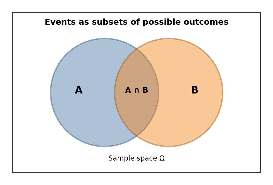
Fig. 1 Events are subsets of the sample space. The overlap \(A \cap B\) is the event that both \(A\) and \(B\) occur.

For any event \(A\), its probability satisfies:

\[ 0 \leq P(A) \leq 1 \]

The impossible event has probability 0, the entire sample space has probability 1, and larger probabilities mean greater likelihood.

The Frequentist Approach

The frequentist interpretation treats probability as a long-run relative frequency. If we repeat the same experiment many times under the same conditions, the probability of an event is the proportion of times that event occurs in the long run.

For example, if a coin is fair, the frequentist interpretation says:

\[ P(\text{heads}) = 0.5 \]

because the fraction of heads should approach \(0.5\) as the number of tosses becomes very large.

This interpretation is useful for repeatable processes: coin flips, manufacturing defects, randomized experiments, survey sampling, A/B tests, and simulations. It is less straightforward for one-time events, such as “this exact bridge will fail this year” or “this candidate will win this election,” because the event is not literally repeated under identical conditions.

Discrete Probability Basics

A probability model is discrete when its possible outcomes form a finite or countably infinite set. Examples include the number of GPS satellites visible to a UAV, the number of obstacles detected during a flight, or a flight-mode status selected from a fixed list.

Suppose a UAV classifies the wind condition during the next control interval as one of three outcomes:

\[ \Omega = \{\text{calm},\text{moderate},\text{strong}\}. \]

Based on recent measurements, assume the probabilities are:

Outcome \(x\)	\(P(X=x)\)
Calm	\(0.50\)
Moderate	\(0.35\)
Strong	\(0.15\)

Each probability must be nonnegative, and the probabilities of all possible outcomes must sum to 1:

\[ 0.50+0.35+0.15=1. \]

For a discrete outcome, the probability of an event is found by adding the probabilities of the outcomes belonging to that event. Let \(A\) be the event that the wind is not calm:

\[ A=\{\text{moderate},\text{strong}\}. \]

Then:

\[ P(A)=P(X=\text{moderate})+P(X=\text{strong}) =0.35+0.15=0.50. \]

The complement \(A^c\) contains every outcome not in \(A\). Therefore:

\[ P(A^c)=1-P(A). \]

In this example, \(A^c\) is the event that the wind is calm, so \(P(A^c)=1-0.50=0.50\).

When all outcomes are equally likely, probability can also be computed by counting:

\[ P(A)=\frac{\text{number of outcomes in }A} {\text{total number of outcomes}}. \]

This counting shortcut applies to a fair die or a well-shuffled deck, but it would not apply to the wind example because its three outcomes have different probabilities. Once additional information is observed, such as a strong-wind warning from a nearby weather station, we use conditional probability to update these probabilities.

Conditional Discrete Probability

Conditional probability asks how probabilities change after we restrict attention to a condition.

For events:

\[ P(A \mid B)=\frac{P(A \cap B)}{P(B)} \qquad \text{if } P(B)>0 \]

For discrete random variables:

\[ P(X=x \mid Y=y)=\frac{P(X=x, Y=y)}{P(Y=y)} \qquad \text{if } P(Y=y)>0 \]

Example: roll two fair dice. Let:

• \(X =\) value of the first die.

• \(S =\) sum of both dice.

What is \(P(X=4 \mid S=7)\)?

The outcomes with sum 7 are:

\[ (1,6),(2,5),(3,4),(4,3),(5,2),(6,1) \]

There are 6 equally likely outcomes under the condition \(S=7\). Only one has \(X=4\), namely \((4,3)\). Therefore:

\[ P(X=4 \mid S=7)=\frac16 \]

Now ask a different question: what is \(P(X \geq 4 \mid S=7)\)?

The favorable outcomes are:

\[ (4,3),(5,2),(6,1) \]

So:

\[ P(X \geq 4 \mid S=7)=\frac{3}{6}=\frac12 \]

Conditional probability is the foundation for Bayes’ rule, Markov chains, many machine learning models, and statistical inference.

Rules of Probability

Two rules appear constantly: the sum rule and the product rule.

Sum Rule

For any two events \(A\) and \(B\):

\[ P(A \cup B) = P(A) + P(B) - P(A \cap B) \]

We subtract \(P(A \cap B)\) because the overlap gets counted twice when we add \(P(A)\) and \(P(B)\).

If \(A\) and \(B\) are mutually exclusive, meaning they cannot both happen, then \(P(A \cap B)=0\) and:

\[ P(A \cup B) = P(A) + P(B) \]

Product Rule

The product rule connects joint probability and conditional probability:

\[ P(A \cap B) = P(A \mid B)P(B) \]

Equivalently:

\[ P(A \cap B) = P(B \mid A)P(A) \]

If \(A\) and \(B\) are independent, then learning that one happened does not change the probability of the other. In that case:

\[ P(A \cap B) = P(A)P(B) \]

Bayes’ Rule

Bayes’ rule is a way to reverse a conditional probability. It follows directly from the product rule:

\[ P(A \mid B) = \frac{P(B \mid A)P(A)}{P(B)} \]

The pieces have useful names:

• \(P(A)\) is the prior probability of \(A\).

• \(P(B \mid A)\) is the likelihood of observing evidence \(B\) if \(A\) is true.

• \(P(B)\) is the evidence or normalizing probability.

• \(P(A \mid B)\) is the posterior probability of \(A\) after observing \(B\).

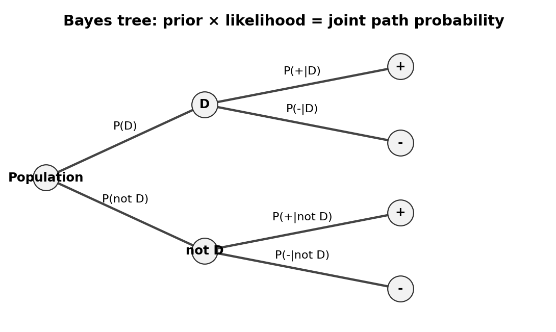
Fig. 2 A probability tree helps track joint probabilities. Each full path multiplies the probabilities along its branches.

Example: suppose a disease affects 1% of a population. A test is positive 95% of the time when a person has the disease and positive 5% of the time when a person does not have it. What is \(P(D \mid +)\), the probability a person has the disease given a positive test?

\[ P(D \mid +) = \frac{P(+ \mid D)P(D)} {P(+ \mid D)P(D) + P(+ \mid D^c)P(D^c)} \]

Substitute:

\[ P(D \mid +) = \frac{0.95 \cdot 0.01} {0.95 \cdot 0.01 + 0.05 \cdot 0.99} = \frac{0.0095}{0.059} \approx 0.161 \]

Even with a positive test, the probability is about 16.1%, because the disease is rare and false positives matter.

Discrete Random Variables

A random variable is a function that assigns a numerical value to each outcome of a random experiment. A discrete random variable takes values in a finite or countably infinite set.

Examples:

• \(X =\) number of heads in 3 coin flips, so \(X \in \{0,1,2,3\}\).

• \(Y =\) result of a die roll, so \(Y \in \{1,2,3,4,5,6\}\).

• \(N =\) number of emails received in an hour, so \(N \in \{0,1,2,\ldots\}\).

For a discrete random variable \(X\), the probability mass function or PMF is:

\[ p(x) = P(X=x) \]

The PMF must satisfy:

\[ p(x) \geq 0 \qquad \text{and} \qquad \sum_x p(x) = 1 \]

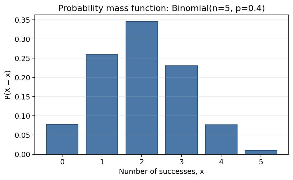
Fig. 3 A PMF assigns probability to each possible value of a discrete random variable.

Common Types of Discrete Random Variables

Several discrete distributions appear so often that they are worth recognizing.

Distribution	Values	Typical use	PMF
Bernoulli\((p)\)	\(0,1\)	One yes/no trial	\(P(X=1)=p\), \(P(X=0)=1-p\)
Binomial\((n,p)\)	\(0,1,\ldots,n\)	Number of successes in \(n\) independent Bernoulli trials	\(P(X=k)=\binom{n}{k}p^k(1-p)^{n-k}\)
Geometric\((p)\)	\(1,2,\ldots\)	Trial number of the first success	\(P(X=k)=(1-p)^{k-1}p\)
Poisson\((\lambda)\)	\(0,1,2,\ldots\)	Counts in a fixed time or space interval	\(P(X=k)=e^{-\lambda}\lambda^k/k!\)
Discrete uniform	finite set	Equally likely outcomes	\(P(X=x)=1/n\) for \(n\) outcomes

The distribution you choose should reflect the data-generating process. For example, a Binomial model assumes a fixed number of trials, two outcomes per trial, constant success probability, and independence.

Example 1: Defective Parts

A factory produces parts. Each part is defective with probability \(p=0.02\), independently of the others. If we inspect \(n=10\) parts, let:

\[ X = \text{number of defective parts} \]

Then:

\[ X \sim \text{Binomial}(10, 0.02) \]

What is the probability of finding exactly one defective part?

\[ P(X=1)=\binom{10}{1}(0.02)^1(0.98)^9 \]

\[ P(X=1)=10(0.02)(0.98)^9 \approx 0.1667 \]

So there is about a 16.7% chance of exactly one defective part.

What is the probability of at least one defective part?

It is easier to use the complement:

\[ P(X \geq 1) = 1 - P(X=0) \]

\[ P(X \geq 1) = 1 - \binom{10}{0}(0.02)^0(0.98)^{10} \]

\[ P(X \geq 1) = 1 - 0.98^{10} \approx 0.1829 \]

So there is about an 18.3% chance of at least one defective part.

Example 2: Help Desk Tickets

Suppose the number of support tickets arriving in an hour is modeled as:

\[ X \sim \text{Poisson}(3) \]

Here \(\lambda=3\) means the expected number of tickets per hour is 3.

What is the probability of exactly 5 tickets?

\[ P(X=5)=e^{-3}\frac{3^5}{5!} \]

\[ P(X=5)=e^{-3}\frac{243}{120}\approx 0.1008 \]

What is the probability of at most 2 tickets?

\[ P(X \leq 2)=P(X=0)+P(X=1)+P(X=2) \]

\[ P(X \leq 2)=e^{-3}\frac{3^0}{0!}+e^{-3}\frac{3^1}{1!}+e^{-3}\frac{3^2}{2!} \]

\[ P(X \leq 2)=e^{-3}(1+3+4.5)\approx 0.4232 \]

So the probability of at most 2 tickets in an hour is about 42.3%.

Expectation and Variance

The expectation of a discrete random variable is its probability-weighted average:

\[ E[X] = \sum_x xP(X=x) \]

Expectation is not necessarily a value that \(X\) can actually take. A fair die has:

\[ E[X] = 1\cdot\frac16 + 2\cdot\frac16 + \cdots + 6\cdot\frac16 = 3.5 \]

No die roll is 3.5, but 3.5 is the long-run average roll.

The variance measures spread around the expectation:

\[ \operatorname{Var}(X) = E[(X-E[X])^2] \]

For a discrete random variable:

\[ \operatorname{Var}(X) = \sum_x (x-\mu)^2P(X=x) \qquad \text{where } \mu=E[X] \]

A useful equivalent formula is:

\[ \operatorname{Var}(X)=E[X^2]-(E[X])^2 \]

where:

\[ E[X^2]=\sum_x x^2P(X=x) \]

For common distributions:

Distribution	\(E[X]\)	\(\operatorname{Var}(X)\)
Bernoulli\((p)\)	\(p\)	\(p(1-p)\)
Binomial\((n,p)\)	\(np\)	\(np(1-p)\)
Geometric\((p)\)	\(1/p\)	\((1-p)/p^2\)
Poisson\((\lambda)\)	\(\lambda\)	\(\lambda\)

Summary

Probability starts with a sample space and events. Venn diagrams help visualize event relationships, while the sum and product rules let us calculate compound probabilities. Bayes’ rule updates beliefs using evidence. Discrete random variables turn outcomes into numbers, PMFs assign probabilities to those numbers, and expectation and variance summarize center and spread. Conditional probability ties all of these ideas together by showing how probabilities change when new information is known.

Practice Questions and Solutions

1. Probability and Conditional Probability: Obstacle Detection

During a UAV flight, the probability that an obstacle is present in the planned path is \(0.10\). The onboard detector raises an alert with probability \(0.90\) when an obstacle is present. When no obstacle is present, it still raises a false alert with probability \(0.05\).

1. What is the probability that the detector raises an alert?

2. If the detector raises an alert, what is the probability that an obstacle is actually present?

2. Discrete Random Variable: Telemetry Packets

A UAV transmits five telemetry packets during a maneuver. Each packet is received successfully with probability \(0.80\), independently of the other packets. Let \(X\) be the number of packets received successfully.

1. What distribution does \(X\) follow?

2. What is the probability that at least four packets are received successfully?

3. Find \(E[X]\) and \(\operatorname{Var}(X)\).

3. Discrete Random Variable: Wind Gusts

The number of unexpected strong wind gusts encountered during a UAV flight is modeled as a Poisson random variable with an average of two gusts per flight. Let \(Y\) be the number of gusts.

1. What is the probability that the UAV encounters at most one gust?

2. What are the expected value and variance of \(Y\)?

4. Mean and Variance: GPS Lock Acquisition

Before beginning a mission, a UAV repeatedly scans for a reliable GPS lock. Each scan succeeds with probability \(0.75\), independently of previous scans. Let \(Z\) be the number of scans required to obtain the first reliable GPS lock, including the successful scan.

1. What distribution does \(Z\) follow?

2. Find \(E[Z]\) and \(\operatorname{Var}(Z)\).

3. Briefly interpret the expected value in the context of the UAV mission.

References

• Joseph K. Blitzstein and Jessica Hwang, Introduction to Probability, 2nd ed., CRC Press, 2019. Book site: https://projects.iq.harvard.edu/stat110/home

• OpenStax, Introductory Statistics, probability and discrete random variable chapters: https://openstax.org/details/books/introductory-statistics

• Joseph Bertrand, Calcul des probabilités, 1889. See overview of Bertrand’s chord paradox: https://en.wikipedia.org/wiki/Bertrand_paradox_(probability)

• Richard von Mises, frequentist interpretation overview: https://plato.stanford.edu/entries/probability-interpret/

• An exceptional set of lectures on probability and statistics by Steven Brunton of UWash: https://youtube.com/playlist?list=PLMrJAkhIeNNR3sNYvfgiKgcStwuPSts9V&si=sFO1lSGlWPbBZHzg/

• Companion code notebook for plotting the discrete probability distributions: discrete probability plotting notebook