
Signal Temporal Logic for UAV Behavior#
This notebook is a hands-on introduction to Signal Temporal Logic (STL). You will build a small STL checker from scratch and use it to reason about the behavior of an autonomous fixed-wing UAV over a flight.
STL is the last stop in a logic sequence you have already seen. Boolean and propositional logic reason about facts that are either true or false. Linear Temporal Logic (LTL) adds time, but still over discrete states and true/false values. STL goes two steps further:
It works on real-valued signals sampled over continuous time, such as altitude in meters or battery percentage, instead of abstract atomic propositions.
Its temporal operators carry explicit time bounds, so you can say “within the next 30 seconds” rather than just “eventually”.
We use the same temporal operator symbols you met in LTL:
G (globally) means “always”, the property holds at every instant in the window.
F (finally) means “eventually”, the property holds at some instant in the window.
U (until) means one property holds continuously until a second one becomes true.
In STL each of these carries a time interval, written as a subscript, for example \(G_{[0,120]}\) or \(F_{[0,30]}\).
The idea you should take away is robustness. Instead of only answering “did the flight satisfy the specification, yes or no”, STL gives a real number that measures how strongly the specification held or how badly it failed. Positive means satisfied with margin, negative means violated, and the magnitude is the size of the margin.
1. Signals#
An STL signal is a real-valued quantity sampled over time. We represent a signal as a
NumPy array of values aligned to a shared time vector t. A flight is just a dictionary
of named signals that all share the same time base.
Below we build a simple simulated mission for one UAV:
alt: altitude in meters. The aircraft climbs, cruises, then descends back down.dist: horizontal distance from the home/launch point in meters. It flies out and returns.batt: battery state of charge as a percentage, draining over the flight.
These are hand-built here so the notebook runs anywhere, but the same code works on logged flight data.
import numpy as np
import matplotlib.pyplot as plt

# Time base: 120 second flight sampled every 0.5 s
dt = 0.5
t = np.arange(0.0, 120.0 + dt, dt)

def ramp(t, t0, t1, v0, v1):
    # Linear segment from v0 at t0 to v1 at t1, held flat outside the interval.
    y = np.clip((t - t0) / (t1 - t0), 0.0, 1.0)
    return v0 + (v1 - v0) * y

# Altitude: climb to 110 m by t=25, cruise, descend to 5 m by t=110
alt = np.where(t < 80, ramp(t, 0, 25, 0, 110), ramp(t, 80, 110, 110, 5))

# Horizontal distance from home: fly out to ~200 m, then return under 10 m by the end
dist = np.where(t < 60, ramp(t, 0, 55, 0, 200), ramp(t, 60, 108, 200, 4))

# Battery: drains from 100% to about 34%
batt = ramp(t, 0, 120, 100, 34)

flight = {"t": t, "alt": alt, "dist": dist, "batt": batt}

print("samples:", len(t))
print("altitude range:  %.1f to %.1f m" % (alt.min(), alt.max()))
print("distance range:  %.1f to %.1f m" % (dist.min(), dist.max()))
print("battery range:   %.1f to %.1f %%" % (batt.min(), batt.max()))
samples: 241
altitude range:  0.0 to 110.0 m
distance range:  0.0 to 200.0 m
battery range:   34.0 to 100.0 %
Let us plot the three signals so we can see the mission before we reason about it.
fig, axes = plt.subplots(3, 1, figsize=(9, 7), sharex=True)

axes[0].plot(t, alt, color="tab:blue")
axes[0].axhline(120, color="tab:red", ls="--", lw=1, label="geofence ceiling 120 m")
axes[0].set_ylabel("altitude (m)")
axes[0].legend(loc="upper right")

axes[1].plot(t, dist, color="tab:green")
axes[1].axhline(10, color="tab:red", ls="--", lw=1, label="home radius 10 m")
axes[1].set_ylabel("dist from home (m)")
axes[1].legend(loc="upper right")

axes[2].plot(t, batt, color="tab:orange")
axes[2].axhline(20, color="tab:red", ls="--", lw=1, label="min battery 20%")
axes[2].set_ylabel("battery (%)")
axes[2].set_xlabel("time (s)")
axes[2].legend(loc="upper right")

fig.suptitle("Simulated UAV mission")
fig.tight_layout()
plt.show()
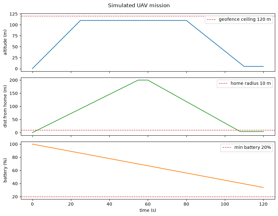
2. Atomic predicates and robustness#
The smallest piece of an STL formula is an atomic predicate: a comparison between a
signal and a constant, such as alt <= 120. In classic logic this is just true or
false at each instant. In STL we instead compute a robustness value at each instant.
The convention is to write every predicate in the form f(signal) >= 0 and let the
robustness be the value of f itself:
For
signal >= c, robustness issignal - c.For
signal <= c, robustness isc - signal.
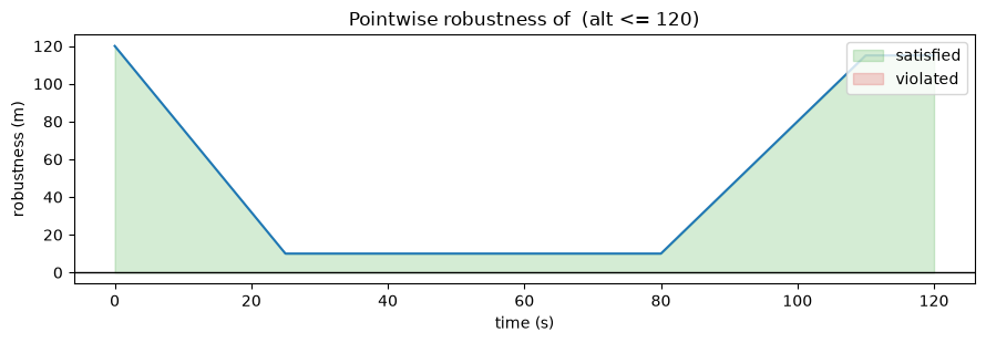
So alt <= 120 has robustness 120 - alt. When the altitude is 110, the robustness is
+10, meaning the predicate holds with 10 m of margin. If the altitude were 128, the
robustness would be -8, meaning it failed by 8 m.
A predicate here is a Python function that takes a flight dictionary and returns a robustness array over time.
def geq(name, c):
    "Predicate: signal >= c.  Robustness = signal - c."
    return lambda s: s[name] - c

def leq(name, c):
    "Predicate: signal <= c.  Robustness = c - signal."
    return lambda s: c - s[name]

# Example: altitude stays under the 120 m ceiling
under_ceiling = leq("alt", 120)
rho = under_ceiling(flight)

print("robustness of (alt <= 120) at a few times:")
for ti in [0, 25, 60, 110]:
    i = int(ti / dt)
    print("  t=%3d s:  alt=%6.1f m   robustness=%+6.1f" % (t[i], alt[i], rho[i]))
robustness of (alt <= 120) at a few times:
  t=  0 s:  alt=   0.0 m   robustness=+120.0
  t= 25 s:  alt= 110.0 m   robustness= +10.0
  t= 60 s:  alt= 110.0 m   robustness= +10.0
  t=110 s:  alt=   5.0 m   robustness=+115.0
Notice the robustness is an array, one value per time sample. It is positive everywhere here because the altitude never reaches the ceiling. The tightest point is during cruise, where the margin shrinks to about 10 m.
plt.figure(figsize=(9, 3.2))
plt.plot(t, rho, color="tab:blue")
plt.axhline(0, color="k", lw=1)
plt.fill_between(t, rho, 0, where=(rho >= 0), color="tab:green", alpha=0.2, label="satisfied")
plt.fill_between(t, rho, 0, where=(rho < 0), color="tab:red", alpha=0.2, label="violated")
plt.title("Pointwise robustness of  (alt <= 120)")
plt.xlabel("time (s)"); plt.ylabel("robustness (m)")
plt.legend(loc="upper right")
plt.tight_layout(); plt.show()
3. Boolean operators#
STL combines predicates with the usual Boolean operators, but on robustness values the operators become min, max, and negation:
not phihas robustness-rho(phi).phi1 and phi2has robustnessmin(rho1, rho2), the weaker of the two.phi1 or phi2has robustnessmax(rho1, rho2), the stronger of the two.
The and rule matches intuition. A conjunction is only as satisfied as its weakest
part, so we take the minimum margin.
def Not(phi):
    return lambda s: -phi(s)

def And(*phis):
    return lambda s: np.min(np.stack([p(s) for p in phis]), axis=0)

def Or(*phis):
    return lambda s: np.max(np.stack([p(s) for p in phis]), axis=0)

# Safe envelope at each instant: under the ceiling AND above 20% battery
safe_now = And(leq("alt", 120), geq("batt", 20))
r_safe = safe_now(flight)
print("min robustness of the instantaneous safe envelope: %+.1f" % r_safe.min())
print("(positive means the envelope held at every sample)")
min robustness of the instantaneous safe envelope: +10.0
(positive means the envelope held at every sample)
4. Temporal operators: G, F, and U#
This is where STL earns its name. Each temporal operator carries a time interval
[a, b] measured in seconds relative to the current instant.
G (globally / always). \(G_{[a,b]}\,\varphi\) holds at time t if \(\varphi\) holds at
every instant in [t+a, t+b]. On robustness values this is a minimum over that
window, since the weakest instant decides whether the property held throughout.
F (finally / eventually). \(F_{[a,b]}\,\varphi\) holds at time t if \(\varphi\) holds
at some instant in [t+a, t+b]. On robustness values this is a maximum over that
window, since one good instant is enough.
U (until). \(\varphi_1\,U_{[a,b]}\,\varphi_2\) holds at time t if there is some
instant \(t'\) in [t+a, t+b] where \(\varphi_2\) becomes true, and \(\varphi_1\) holds
continuously from t up to that instant. On robustness values it is a max over the
possible switch points \(t'\), and at each \(t'\) we take the min of the robustness of
\(\varphi_2\) at \(t'\) and the smallest robustness of \(\varphi_1\) over the run-up. This
nesting of min and max is why until is the richest of the three.
We implement each operator as a sliding window over the robustness arrays. The interval
in seconds is converted to a number of samples using dt.
def G(phi, interval, dt):
    "Globally / always over [a, b]."
    a, b = interval
    ia, ib = int(round(a / dt)), int(round(b / dt))
    def f(s):
        rho = phi(s)
        n = len(rho)
        out = np.full(n, np.inf)
        for i in range(n):
            lo, hi = i + ia, min(i + ib, n - 1)
            if lo <= n - 1:
                out[i] = np.min(rho[lo:hi + 1])
        return out
    return f

def F(phi, interval, dt):
    "Finally / eventually over [a, b]."
    a, b = interval
    ia, ib = int(round(a / dt)), int(round(b / dt))
    def f(s):
        rho = phi(s)
        n = len(rho)
        out = np.full(n, -np.inf)
        for i in range(n):
            lo, hi = i + ia, min(i + ib, n - 1)
            if lo <= n - 1:
                out[i] = np.max(rho[lo:hi + 1])
        return out
    return f

def U(phi1, phi2, interval, dt):
    "phi1 Until phi2 over [a, b]."
    a, b = interval
    ia, ib = int(round(a / dt)), int(round(b / dt))
    def f(s):
        r1, r2 = phi1(s), phi2(s)
        n = len(r1)
        out = np.full(n, -np.inf)
        for i in range(n):
            best = -np.inf
            for j in range(max(i + ia, 0), min(i + ib, n - 1) + 1):
                hold = np.min(r1[i:j + 1])      # phi1 must hold from now up to t'
                best = max(best, min(r2[j], hold))
            out[i] = best
        return out
    return f

def robustness(phi, s, at_time=0.0):
    "Robustness of the whole formula, read at a single instant (default t=0)."
    i = int(round(at_time / dt))
    return phi(s)[i]

def verdict(phi, s, at_time=0.0):
    r = robustness(phi, s, at_time)
    return ("SATISFIED" if r >= 0 else "VIOLATED"), r
A note on the window at the end of the flight: when the interval [t+a, t+b]
runs past the last sample, we shrink it to whatever samples remain. For the whole-flight
specifications below we read the result at t = 0 with an interval that spans the full
horizon, so this edge case does not affect the verdict.
5. UAV specifications#
Now we write real mission requirements as STL formulas and check them against the
flight. Each one is read at t = 0, so the interval covers the part of the flight we
care about.
Spec 1. Geofence ceiling. The altitude must never exceed 120 m for the entire flight.
phi1 = G(leq("alt", 120), (0, 120), dt)
print("Spec 1  geofence ceiling:      %s  (robustness %+.1f m)" % verdict(phi1, flight))
Spec 1 geofence ceiling: SATISFIED (robustness +10.0 m)
Spec 2. Reach cruise altitude promptly. The aircraft must climb above 100 m at some point within the first 30 seconds.
phi2 = F(geq("alt", 100), (0, 30), dt)
print("Spec 2  reach 100 m by t=30:   %s  (robustness %+.1f m)" % verdict(phi2, flight))
Spec 2 reach 100 m by t=30: SATISFIED (robustness +10.0 m)
Spec 3. Battery floor. The battery must stay at or above 20% for the whole flight.
phi3 = G(geq("batt", 20), (0, 120), dt)
print("Spec 3  battery >= 20%%:        %s  (robustness %+.1f %%)" % verdict(phi3, flight))
Spec 3 battery >= 20%: SATISFIED (robustness +14.0 %)
Spec 4. Return to launch. The aircraft must come back to within 10 m of home at some point in the final 20 seconds.
phi4 = F(leq("dist", 10), (100, 120), dt)
print("Spec 4  return within 10 m:    %s  (robustness %+.1f m)" % verdict(phi4, flight))
Spec 4 return within 10 m: SATISFIED (robustness +6.0 m)
Spec 5. Stay inside the geofence until home. Using until, we require the altitude to remain under the 120 m ceiling continuously until the aircraft is back within 10 m of home. The until captures the ordering: the ceiling constraint must hold right up to the moment the return condition becomes true.
phi5 = U(leq("alt", 120), leq("dist", 10), (0, 120), dt)
print("Spec 5  under ceiling until home:  %s  (robustness %+.1f m)" % verdict(phi5, flight))
Spec 5 under ceiling until home: SATISFIED (robustness +10.0 m)
Spec 6. Full mission. All requirements at once. As a conjunction, its robustness is the minimum of the parts, so it tells you the single tightest margin in the whole mission.
mission = And(phi1, phi2, phi3, phi4, phi5)
status, r = verdict(mission, flight)
print("Full mission spec:  %s  (robustness %+.1f)" % (status, r))
print()
print("The mission robustness equals the smallest of the margins, so it points")
print("straight at the requirement with the least room to spare.")
Full mission spec: SATISFIED (robustness +6.0)
The mission robustness equals the smallest of the margins, so it points
straight at the requirement with the least room to spare.
6. Why robustness is useful#
A plain true/false verdict cannot tell two passing flights apart. Robustness can. Here we tighten the geofence ceiling and watch the same flight go from comfortably safe to a violation, with the robustness reporting exactly how many meters over the limit it went.
for ceiling in [120, 115, 108, 105, 100]:
    spec = G(leq("alt", ceiling), (0, 120), dt)
    status, r = verdict(spec, flight)
    print("ceiling %3d m ->  %-9s  robustness %+6.1f m" % (ceiling, status, r))
ceiling 120 m ->  SATISFIED  robustness  +10.0 m
ceiling 115 m ->  SATISFIED  robustness   +5.0 m
ceiling 108 m ->  VIOLATED   robustness   -2.0 m
ceiling 105 m ->  VIOLATED   robustness   -5.0 m
ceiling 100 m ->  VIOLATED   robustness  -10.0 m
As the ceiling drops toward the cruise altitude the margin shrinks to zero, and once it crosses, the robustness goes negative and reports the size of the overshoot. This is what makes STL robustness valuable for tuning controllers, comparing runs, and using the margin as a reward signal in learning based control.
Summary#
You built a working STL checker in a few dozen lines and used it to reason about a UAV mission. The pieces were: signals as real-valued arrays over time, atomic predicates that produce a signed margin instead of a bare true/false, Boolean operators that become min, max, and negation on those margins, and the time-bounded temporal operators G, F, and U built as sliding min and max windows over those margins. The single most important idea is robustness: STL does not just tell you whether a flight met its specification, it tells you by how much, which is exactly the quantity you want when tuning, comparing, or learning controllers.